Linear Regression
Foreword
We begin to dive into the world of actual Machine Learning starting from this topic. There are few techniques of ML: Supervised Learning, Unsupervised Learning, Reinforcement Learning and Semi-supervised Learning. And Linear Regression is one of the bases of "Supervised Learning" techniques.
What is Linear Regression?
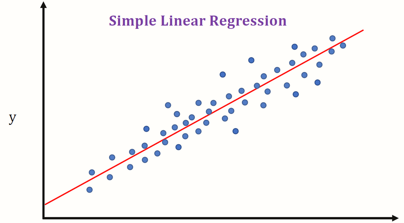
Linear regression is a model that assumes a relationship between the independent(x) variables and one dependent(y) variable. It performs the task to predict a dependent(y) variable value based on a given independent(x) variable. Simple linear regression is a type of linear regression where there is single independent(x) variable.
Let us understand the principle of the regression model visually with the help of a video published in channel StatQuest with Josh Starmer
Now let's have a look at the post published in Towards Data Science by Rohith Gandhi
y = a_0 + a_1 * x ## Linear Equation
The motive of the linear regression algorithm is to find the best values for a_0 and a_1. Before moving on to the algorithm, let’s have a look at two important concepts you must know to better understand linear regression.
Cost Function
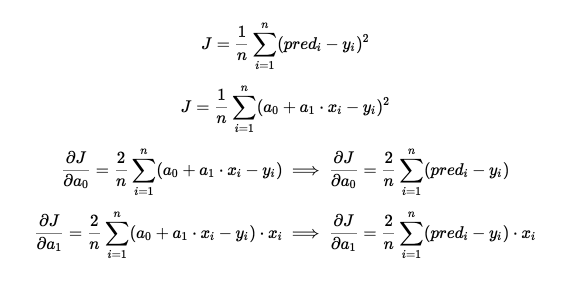
The cost function helps us to figure out the best possible values for a_0 and a_1 which would provide the best fit line for the data points. Since we want the best values for a_0 and a_1, we convert this search problem into a minimization problem where we would like to minimize the error between the predicted value and the actual value.
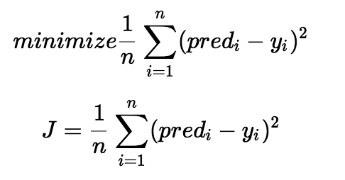
We choose the above function to minimize. The difference between the predicted values and ground truth measures the error difference. We square the error difference and sum over all data points and divide that value by the total number of data points. This provides the average squared error over all the data points. Therefore, this cost function is also known as the Mean Squared Error(MSE) function. Now, using this MSE function we are going to change the values of a_0 and a_1 such that the MSE value settles at the minima.
Gradient Descent
The next important concept needed to understand linear regression is gradient descent. Gradient descent is a method of updating a_0 and a_1 to reduce the cost function(MSE). The idea is that we start with some values for a_0 and a_1 and then we change these values iteratively to reduce the cost. Gradient descent helps us on how to change the values.
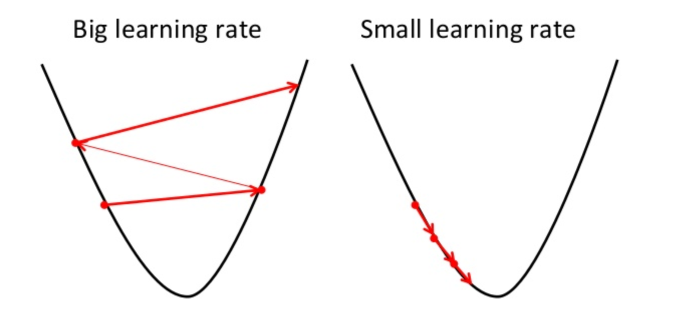
To draw an analogy, imagine a pit in the shape of U and you are standing at the topmost point in the pit and your objective is to reach the bottom of the pit. There is a catch, you can only take a discrete number of steps to reach the bottom. If you decide to take one step at a time you would eventually reach the bottom of the pit but this would take a longer time. If you choose to take longer steps each time, you would reach sooner but, there is a chance that you could overshoot the bottom of the pit and not exactly at the bottom. In the gradient descent algorithm, the number of steps you take is the learning rate. This decides on how fast the algorithm converges to the minima.
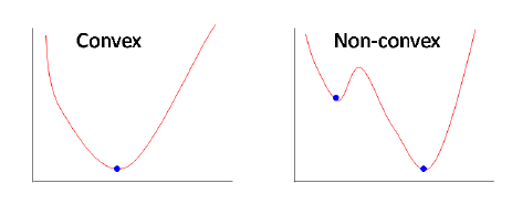
Sometimes the cost function can be a non-convex function where you could settle at a local minima but for linear regression, it is always a convex function.
You may be wondering how to use gradient descent to update a_0 and a_1. To update a_0 and a_1, we take gradients from the cost function. To find these gradients, we take partial derivatives with respect to a_0 and a_1. Now, to understand how the partial derivatives are found below you would require some calculus but if you don’t, it is alright. You can take it as it is.
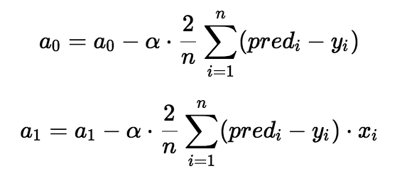
The partial derivates are the gradients and they are used to update the values of a_0 and a_1. Alpha is the learning rate which is a hyperparameter that you must specify. A smaller learning rate could get you closer to the minima but takes more time to reach the minima, a larger learning rate converges sooner but there is a chance that you could overshoot the minima.
The article is very well written, I advice you to visit at the end https://towardsdatascience.com/introduction-to-machine-learning-algorithms-linear-regression-14c4e325882a
As I guess, video explanation would make a better picture. The ML video-tutorial from codebasics would be suitable for our topic.
import numpy as np

def gradient_descent(x,y):
    m_curr = b_curr = 0
    iterations = 10000
    n = len(x)
    learning_rate = 0.08

    for i in range(iterations):
        y_predicted = m_curr * x + b_curr
        cost = (1/n) * sum([val**2 for val in (y-y_predicted)])
        md = -(2/n)*sum(x*(y-y_predicted))
        bd = -(2/n)*sum(y-y_predicted)
        m_curr = m_curr - learning_rate * md
        b_curr = b_curr - learning_rate * bd
        print ("m {}, b {}, cost {} iteration {}".format(m_curr,b_curr,cost, i))

x = np.array([1,2,3,4,5])
y = np.array([5,7,9,11,13])

gradient_descent(x,y)
References
https://towardsdatascience.com/introduction-to-machine-learning-algorithms-linear-regression-14c4e325882a
https://machinelearningmastery.com/linear-regression-for-machine-learning/