Hypothesis Testing: 1-Tailed Test With t-Distribution

In this article, I want to demonstrate the use of the 1-Tailed test using the t-distribution. When is this test required rather than using the z-distribution test which we have looked at in previous articles?

The problem that I would like to propose for this example is as follows:

Example: The average IQ of the adult population is 100. A researcher believes the average IQ is lower. A random sample of 5 adults are tested and the results tabulated as 69, 79, 89, 99, and 109 with a sample standard deviation of 15.81. Is there enough evidence to suggest that the average IQ is lower than 100?

So, if we look at the steps we should use to work this problem, they are:

1. State the null hypothesis and alternative hypothesis
2. Choose a level of significance
3. Find the critical values
4. Find the test statistic
5. Draw your conclusion.

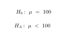
Let's start with step 1. What are the null and alternative hypotheses for this particular example? What is believed to be true is that the average IQ of the adult population is 100. The alternative hypothesis is what is being claimed. In this problem, a researcher believes or is claiming that the average IQ in adults is lower than 100. Therefore, H0 and HA for this problem are as follows:

Anytime a "<" or ">" symbol appears in the alternative hypothesis, we will be using a 1-tailed test for the test statistic. For this problem, a level of confidence or level of significance was not specified. Since the default level of significance in statistical testing is alpha (a = 0.05), we will use that as our value of a. The graph that depicts a normally-distributed data with 1-tailed test where a = 0.05 is shown below:

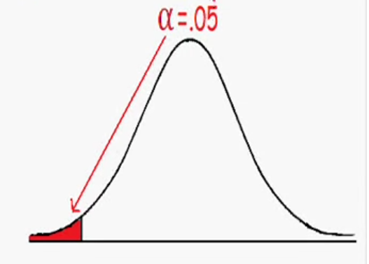
Since the only area of interest in this example for the average IQ in adults is lower than the currently accepted value for the population and we are performing a 1-tailed test, the left-tail of the normal distribution only is selected as our red-shaded area which represents our rejection region. The area of the red region in the left-tail of the graph is also 0.05 corresponding to the value of alpha chosen for this example.

Next, let's move on to step 3 which is to identify the critical values for the problem. The critical values in this problem exist in the area of the curve which is less than the mean population value of 100 at the top of the normal distribution and is the area in the left-tail that separates the red region from the rest of the curve to the right.

The critical values (c.v.) can be either a z-value or a t-value depending on the circumstances in the problem you're testing. For this particular example we're using a t-test instead of a z-test for the following reasons:

In this problem, we are given the standard deviation of 15.81, but this is not sigma, which is the population standard deviation, but instead is the sample standard deviation. So, criteria 1 is met. Secondly, the sample size is given to us as 5 < 30. So, criteria # 2 is met as well. Therefore, we can use the t-test for this problem. When using the t-test, remember that the area under the left-tail of the chart above is 0.05 representing our area of significance. So, pulling out our statistical t-distribution table from the CRC mathematical reference book, we have the following table as shown below:

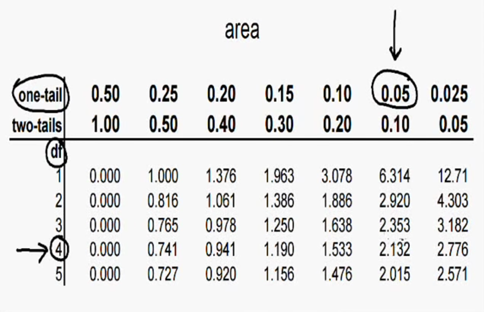
The area of this table that we should focus on is the top row representing a one-tail test rather than the row below which represents a two-tail test. If we go over to the column headed by the value of a = 0.05 and then look down the column to where df (which stands for degrees of freedom) is 4 and where the two intersect is our t-value. In this case, that value is t = 2.132. Why did we choose the degrees of freedom (df) value to be equal to 4 in this example? The degrees of freedom in a t-test is always one less than the sample size we have chosen for the problem. Since we have chosen to sample 5 adults, our df = 5 - 1 = 4. And, since we are concerned with the area shaded in red in the left-tail or left of the average in the chart above, our c.v. = - 2.132 rather than a + 2.132. Now, we need to determine the value of our test statistic, t. The formula for calculating t is:

In this formula X-bar is the average of the IQ scores from our sample, which is (69 + 79 + 89 + 99 + 109) / 5 = 89, mu = population mean, which is 100, s = sample standard deviation = 15.81, and n = sample size = 5. So, plugging all this into the equation above we get:

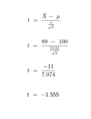
The value of t, therefore, is our test statistic. Rounded to 2-decimal places the value of t = - 1.56. This value for t for this test lies somewhere in the region between our rejection region (shaded red area) and the mean of the population, which is in the center of the chart. Therefore, t does not lie inside the rejection region and we can conclude that we are unable to reject the null hypothesis or we failed to reject H0 and thus we must accept it.

In conclusion, we were asked if there is enough evidence to suggest the average IQ of adults is lower than 100? And the answer to that question is NO. The average IQ remains at 100 with a 95% confidence level.